Using file-backed matrices - FBM • switchgrassGWAS

When you run GWAS using this package, you now have two options for saving the GWAS results - as RDS files and as file-backed matrix (FBM) files.

You can specify this option in pvdiv_standard_gwas() with the option savetype. savetype can be “rds”, “fbm”, or “both”.

Why use RDS files?

If you are running few GWAS and want to save each GWAS output separately, you can use rds files. These files completely describe the GWAS results without referring back to the original SNP file, using the columns CHR (chromosome) & POS (physical position). They contain the effect estimate estim for the alternate allele (allele 2 in the SNP file), the standard error around this effect std_err, and the -log10pvalue and FDR adjusted p-values log10p and FDR_adj from the genome-wide association.

Pros of RDS files

These files are standalone & contain all the information you need to analyze a GWAS result.

These rds files can be used with the function pvdiv_bigsnp2mashr to run mash, as well as with pvdiv_table_topsnps (by specifying type = “bigsnp”), pvdiv_qqplot, and pvdiv_manhattan.

Cons of RDS files

If you are running many GWAS, these files can become numerous, take up substantial disk space, and become hard to keep track of. Individual files make it more difficult to compare results across multiple GWAS.

Why use FBM files?

If you are running many GWAS, you may want a compressed format, a reduced number of files, and/or additional ways to compare GWAS outputs. To do this, you can use FBM files, which save all GWAS results in a total of 4 files. These files all start with the prefix ‘gwas_effects_’. Two are .csv files; these contain the associated metadata for the GWAS and the column names for the fbm. Two are an .rds & .bk format & contain the actual file-backed matrix results; these can be very large.

For each phenotype used for GWAS, the gwas_effects files contain the effect estimate estim for the alternate allele (allele 2 in the SNP file), the standard error around this effect std_err, and the -log10pvalue log10p from the genome-wide association.

Pros of FBM files

FBM files are memory and computation-efficient tools to analyze big matrices that are stored on disc rather than in your computer’s memory (see here for more details ). Briefly, they have faster I/O, won’t overwhelm your computer’s RAM, and function runtime speeds up ~10-200x.

These fbm files can be used with the functions pvdiv_fbm_upset_df() and pvdiv_fbm_qq(). They can also be used in the snpdiver R package function dive_effects2mash() to run mash.

Cons of FBM files

These files need to be used along with the original snp file used to run the GWAS - thus, you’ll need to keep track of six files in total, the .rds and .bk file for the SNP file and the four files for the gwas results.

These files do not work with the function pvdiv_bigsnp2mashr to run mash.

If you are interested in only a subset of GWAS results saved in a fbm, you will have to create a vector of row numbers using the associated metadata to refer to that data subset.

Using FBM gwas results

The remainder of this package demonstrates some utilities for filebacked matrix files within the bigsnpr and switchgrassGWAS R packages.

Get genotype file

# get the example bedfile from the package switchgrassGWAS
bedfile <- system.file("extdata", "example.bed", package = "switchgrassGWAS")

Set up SNP and phenotype data frames.

# Load packages bigsnpr and switchgrassGWAS
library(switchgrassGWAS)
#> Registered S3 method overwritten by 'GGally':
#>   method from   
#>   +.gg   ggplot2
library(bigsnpr)
#> Loading required package: bigstatsr

# Read from bed/bim/fam to create the new files that bigsnpr uses.
# Let's put them in an temporary directory for this demo.
tmpfile <- tempfile()
snp_readBed(bedfile, backingfile = tmpfile)
#> [1] "/tmp/RtmpgAXKt5/file2f365fdb9ef7.rds"

# Attach the "bigSNP" object to the R session.
snp_example <- snp_attach(paste0(tmpfile, ".rds"))
# What does the bigSNP object look like?
str(snp_example, max.level = 2, strict.width = "cut")
#> List of 3
#>  $ genotypes:Reference class 'FBM.code256' [package "bigstatsr"] with 16 fields
#>   ..and 26 methods, of which 12 are  possibly relevant:
#>   ..  add_columns, as.FBM, bm, bm.desc, check_dimensions,
#>   ..  check_write_permissions, copy#envRefClass, initialize, initialize#FBM,
#>   ..  save, show#envRefClass, show#FBM
#>  $ fam      :'data.frame':   630 obs. of  6 variables:
#>   ..$ family.ID  : chr [1:630] "Pvirgatum" "Pvirgatum" "Pvirgatum" "Pvirgatum"..
#>   ..$ sample.ID  : chr [1:630] "J181.A" "J250.C" "J251.C" "J352.A" ...
#>   ..$ paternal.ID: int [1:630] 0 0 0 0 0 0 0 0 0 0 ...
#>   ..$ maternal.ID: int [1:630] 0 0 0 0 0 0 0 0 0 0 ...
#>   ..$ sex        : int [1:630] 0 0 0 0 0 0 0 0 0 0 ...
#>   ..$ affection  : int [1:630] -9 -9 -9 -9 -9 -9 -9 -9 -9 -9 ...
#>  $ map      :'data.frame':   3600 obs. of  6 variables:
#>   ..$ chromosome  : chr [1:3600] "Chr01K" "Chr01K" "Chr01K" "Chr01K" ...
#>   ..$ marker.ID   : chr [1:3600] "Chr01K_105542" "Chr01K_798650" "Chr01K_1147"..
#>   ..$ genetic.dist: int [1:3600] 0 0 0 0 0 0 0 0 0 0 ...
#>   ..$ physical.pos: int [1:3600] 105542 798650 1147074 1719551 1915851 1965986..
#>   ..$ allele1     : chr [1:3600] "A" "C" "T" "T" ...
#>   ..$ allele2     : chr [1:3600] "G" "G" "C" "G" ...
#>  - attr(*, "class")= chr "bigSNP"

# Load the pvdiv phenotypes into the R session.
data(pvdiv_phenotypes) 
# Make an example dataframe of one phenotype where the first column is PLANT_ID.
# This "phenotype", 'GWAS_CT', is the number of times a plant successfully 
# clonally replicated to plant in the common gardens in 2018.
four_phenotype <- pvdiv_phenotypes %>%
  dplyr::select(PLANT_ID, GWAS_CT, matches("BIOMASS"))

Run genome-wide association (GWAS)

# Save the output to a temporary directory for this demo.
tempdir <- tempdir()

pvdiv_standard_gwas(snp = snp_example, df = four_phenotype, 
                    type = "linear", outputdir = tempdir, 
                    savegwas = TRUE, savetype = "fbm", 
                    saveplots = FALSE,
                    saveannos = FALSE, ncores = 1)
#> 'lambdagc' is TRUE, so lambda_GC will be used to find the best population structure correction using the covariance matrix.
#> 'savetype' is 'fbm', so the gwas results will be saved to disk as a combined filebacked matrix (fbm) file.
#> Covariance matrix (covar) was not supplied - this will be generated using pvdiv_autoSVD().
#> 'saveoutput' is FALSE, so the svd will not be saved to the working directory.
#> Now starting GWAS pipeline for GWAS_CT.
#> Now determining lambda_GC for GWAS models with 16 sets of PCs. This will take some time.
#> saveoutput is FALSE, so lambda_GC values won't be saved to a csv.
#> Finished Lambda_GC calculation for GWAS_CT using 0 PCs.
#> Finished Lambda_GC calculation for GWAS_CT using 1 PCs.
#> Finished Lambda_GC calculation for GWAS_CT using 2 PCs.
#> Finished Lambda_GC calculation for GWAS_CT using 3 PCs.
#> Finished Lambda_GC calculation for GWAS_CT using 4 PCs.
#> Finished Lambda_GC calculation for GWAS_CT using 5 PCs.
#> Finished Lambda_GC calculation for GWAS_CT using 6 PCs.
#> Finished Lambda_GC calculation for GWAS_CT using 7 PCs.
#> Finished Lambda_GC calculation for GWAS_CT using 8 PCs.
#> Finished Lambda_GC calculation for GWAS_CT using 9 PCs.
#> Finished Lambda_GC calculation for GWAS_CT using 10 PCs.
#> Finished Lambda_GC calculation for GWAS_CT using 11 PCs.
#> Finished Lambda_GC calculation for GWAS_CT using 12 PCs.
#> Finished Lambda_GC calculation for GWAS_CT using 13 PCs.
#> Finished Lambda_GC calculation for GWAS_CT using 14 PCs.
#> Finished Lambda_GC calculation for GWAS_CT using 15 PCs.
#> Finished phenotype 1: GWAS_CT
#> Now running GWAS with the best population structure correction.
#> [1] "saveoutput is FALSE so GWAS object will not be saved to disk."
#> Now starting GWAS pipeline for CLMB_BIOMASS.
#> Now determining lambda_GC for GWAS models with 16 sets of PCs. This will take some time.
#> saveoutput is FALSE, so lambda_GC values won't be saved to a csv.
#> Finished Lambda_GC calculation for CLMB_BIOMASS using 0 PCs.
#> Finished Lambda_GC calculation for CLMB_BIOMASS using 1 PCs.
#> Finished Lambda_GC calculation for CLMB_BIOMASS using 2 PCs.
#> Finished Lambda_GC calculation for CLMB_BIOMASS using 3 PCs.
#> Finished Lambda_GC calculation for CLMB_BIOMASS using 4 PCs.
#> Finished Lambda_GC calculation for CLMB_BIOMASS using 5 PCs.
#> Finished Lambda_GC calculation for CLMB_BIOMASS using 6 PCs.
#> Finished Lambda_GC calculation for CLMB_BIOMASS using 7 PCs.
#> Finished Lambda_GC calculation for CLMB_BIOMASS using 8 PCs.
#> Finished Lambda_GC calculation for CLMB_BIOMASS using 9 PCs.
#> Finished Lambda_GC calculation for CLMB_BIOMASS using 10 PCs.
#> Finished Lambda_GC calculation for CLMB_BIOMASS using 11 PCs.
#> Finished Lambda_GC calculation for CLMB_BIOMASS using 12 PCs.
#> Finished Lambda_GC calculation for CLMB_BIOMASS using 13 PCs.
#> Finished Lambda_GC calculation for CLMB_BIOMASS using 14 PCs.
#> Finished Lambda_GC calculation for CLMB_BIOMASS using 15 PCs.
#> Finished phenotype 1: CLMB_BIOMASS
#> Now running GWAS with the best population structure correction.
#> [1] "saveoutput is FALSE so GWAS object will not be saved to disk."
#> Now starting GWAS pipeline for KBSM_BIOMASS.
#> Now determining lambda_GC for GWAS models with 16 sets of PCs. This will take some time.
#> saveoutput is FALSE, so lambda_GC values won't be saved to a csv.
#> Finished Lambda_GC calculation for KBSM_BIOMASS using 0 PCs.
#> Finished Lambda_GC calculation for KBSM_BIOMASS using 1 PCs.
#> Finished Lambda_GC calculation for KBSM_BIOMASS using 2 PCs.
#> Finished Lambda_GC calculation for KBSM_BIOMASS using 3 PCs.
#> Finished Lambda_GC calculation for KBSM_BIOMASS using 4 PCs.
#> Finished Lambda_GC calculation for KBSM_BIOMASS using 5 PCs.
#> Finished Lambda_GC calculation for KBSM_BIOMASS using 6 PCs.
#> Finished Lambda_GC calculation for KBSM_BIOMASS using 7 PCs.
#> Finished Lambda_GC calculation for KBSM_BIOMASS using 8 PCs.
#> Finished Lambda_GC calculation for KBSM_BIOMASS using 9 PCs.
#> Finished Lambda_GC calculation for KBSM_BIOMASS using 10 PCs.
#> Finished Lambda_GC calculation for KBSM_BIOMASS using 11 PCs.
#> Finished Lambda_GC calculation for KBSM_BIOMASS using 12 PCs.
#> Finished Lambda_GC calculation for KBSM_BIOMASS using 13 PCs.
#> Finished Lambda_GC calculation for KBSM_BIOMASS using 14 PCs.
#> Finished Lambda_GC calculation for KBSM_BIOMASS using 15 PCs.
#> Finished phenotype 1: KBSM_BIOMASS
#> Now running GWAS with the best population structure correction.
#> [1] "saveoutput is FALSE so GWAS object will not be saved to disk."
#> Now starting GWAS pipeline for PKLE_BIOMASS.
#> Now determining lambda_GC for GWAS models with 16 sets of PCs. This will take some time.
#> saveoutput is FALSE, so lambda_GC values won't be saved to a csv.
#> Finished Lambda_GC calculation for PKLE_BIOMASS using 0 PCs.
#> Finished Lambda_GC calculation for PKLE_BIOMASS using 1 PCs.
#> Finished Lambda_GC calculation for PKLE_BIOMASS using 2 PCs.
#> Finished Lambda_GC calculation for PKLE_BIOMASS using 3 PCs.
#> Finished Lambda_GC calculation for PKLE_BIOMASS using 4 PCs.
#> Finished Lambda_GC calculation for PKLE_BIOMASS using 5 PCs.
#> Finished Lambda_GC calculation for PKLE_BIOMASS using 6 PCs.
#> Finished Lambda_GC calculation for PKLE_BIOMASS using 7 PCs.
#> Finished Lambda_GC calculation for PKLE_BIOMASS using 8 PCs.
#> Finished Lambda_GC calculation for PKLE_BIOMASS using 9 PCs.
#> Finished Lambda_GC calculation for PKLE_BIOMASS using 10 PCs.
#> Finished Lambda_GC calculation for PKLE_BIOMASS using 11 PCs.
#> Finished Lambda_GC calculation for PKLE_BIOMASS using 12 PCs.
#> Finished Lambda_GC calculation for PKLE_BIOMASS using 13 PCs.
#> Finished Lambda_GC calculation for PKLE_BIOMASS using 14 PCs.
#> Finished Lambda_GC calculation for PKLE_BIOMASS using 15 PCs.
#> Finished phenotype 1: PKLE_BIOMASS
#> Now running GWAS with the best population structure correction.
#> [1] "saveoutput is FALSE so GWAS object will not be saved to disk."

This command will save a set of gwas results to a temporary directory, which will have a randomly generated name like: /tmp/RtmpgAXKt5.

Let’s load these files into R.

gwas <- big_attach(file.path(tempdir, "gwas_effects_0M_SNPs.rds"))
gwas_metadata <- read.csv(file.path(tempdir, "gwas_effects_0M_SNPs_associated_metadata.csv"))
gwas_colnames <- read.csv(file.path(tempdir, "gwas_effects_0M_SNPs_column_names.csv"))

Let’s look at the metadata associated with the GWAS. This includes information about the kind of GWAS that was conducted. In order, the columns indicate, what the phenotype name was, what type of model was run, how many SNPs (in M) were used, how many PCs were used for population structure correction, how many phenotyped individuals were there, how many phenotypic levels were there, what was the genomic inflation factor (lambda_GC), and given the number of SNPs, what was the bonferroni threshold for the phenotype.

kable(gwas_metadata)

phe	type	nsnp	npcs	nphe	nlev	lambda_GC	bonferroni
GWAS_CT	linear	0_M	15	629	16	1.12682	4.857333
CLMB_BIOMASS	linear	0_M	5	495	490	1.02958	4.857333
KBSM_BIOMASS	linear	0_M	15	512	512	1.07005	4.857333
PKLE_BIOMASS	linear	0_M	10	612	606	1.03844	4.857333

Let’s look at the column names of the GWAS result. These are in the same order as the associated metadata, and each phenotype has three columns: Effect (estimated effect size of allele2), SE (standard error about this effect size), and log10p (-log10p of the association between SNP & phenotype).

kable(gwas_colnames)

colnames_fbm
GWAS_CT_Effect
GWAS_CT_SE
GWAS_CT_log10p
CLMB_BIOMASS_Effect
CLMB_BIOMASS_SE
CLMB_BIOMASS_log10p
KBSM_BIOMASS_Effect
KBSM_BIOMASS_SE
KBSM_BIOMASS_log10p
PKLE_BIOMASS_Effect
PKLE_BIOMASS_SE
PKLE_BIOMASS_log10p

Two-GWAS Comparisons

Let’s analyze overlaps in significance in the four GWAS. Is there a relationship between the -log10pvalues in the three BIOMASS GWAS? If so, this could indicate that SNPs have a similar effect on BIOMASS across the three different environments.

Use the row numbers from the associated metadata to compare -log10p values for row 2 (CLMB_BIOMASS) with rows 3 & 4 (biomass at KBSM & PKLE). Set the threshold above which to plot the p-value at zero (default is 5), because there are not many SNPs in this toy example.

pvdiv_fbm_qq(effects = gwas, metadata = gwas_metadata, e_row = 2, o_row = 3:4, 
             outputdir = tempdir, thr = 0)
#> `geom_smooth()` using method = 'gam' and formula 'y ~ s(x, bs = "cs")'
#> `geom_smooth()` using method = 'gam' and formula 'y ~ s(x, bs = "cs")'

This function will again save plots to the tempdir. These plots should look like this:

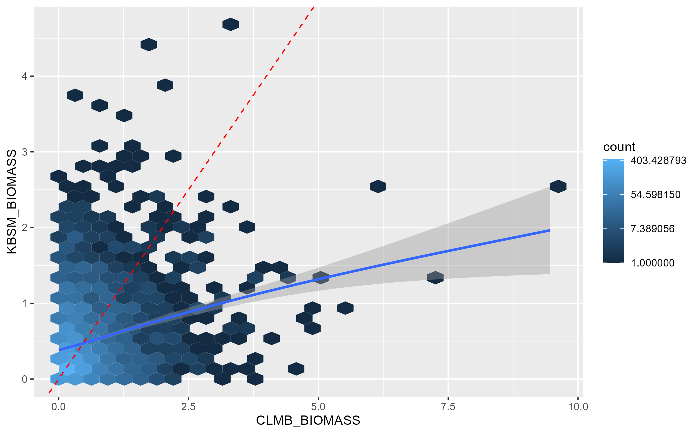
CLMB_vs_KBSM

and this:

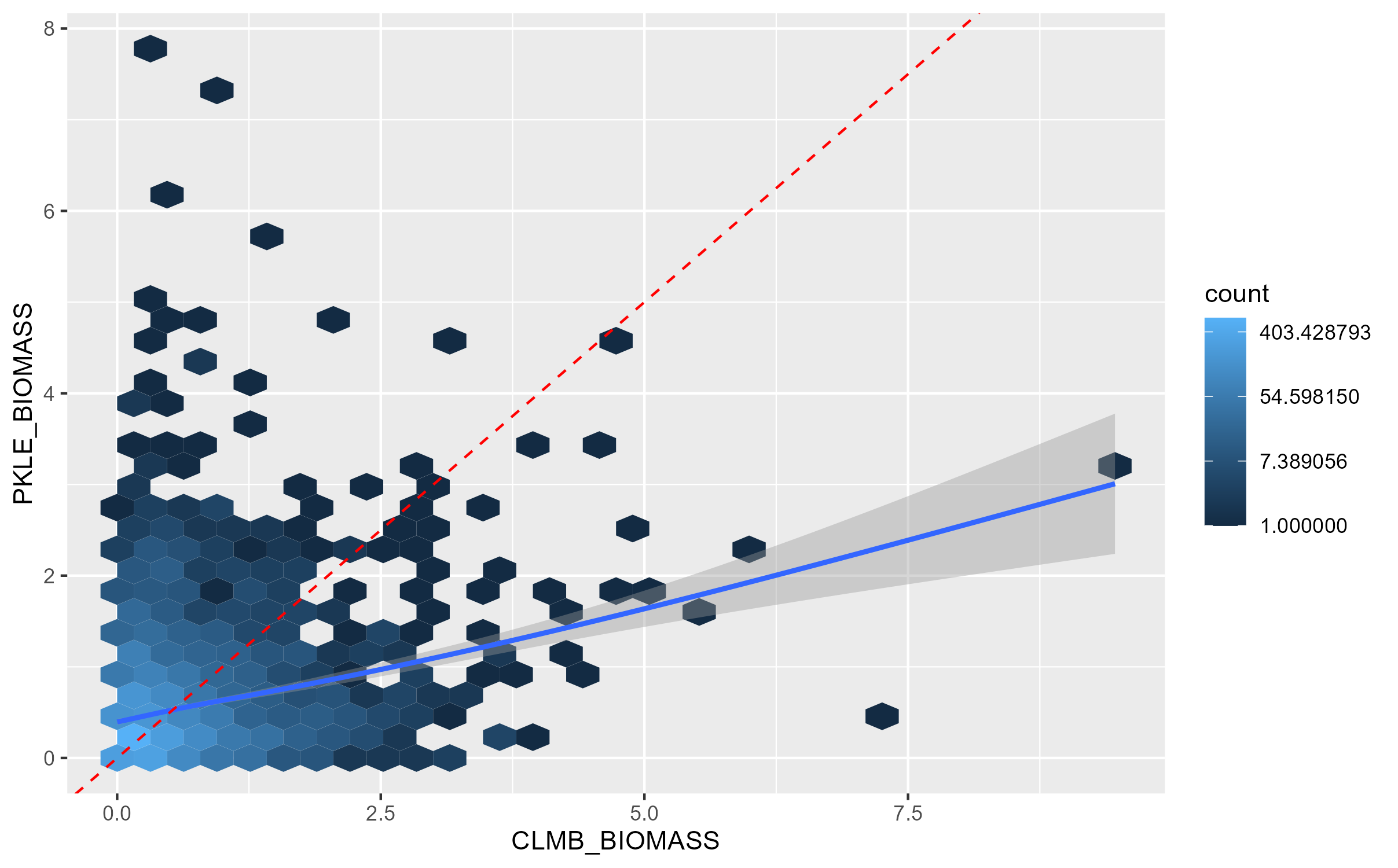
CLMB_vs_PKLE

If these GWAS results were perfectly related, all the hexagons would fall on the red dashed 1:1 line. The blue line indicates the actual relationship between the p-values in the two GWAS. We can see that there is a modest positive relationship between biomass in these environments, but it’s by no means strong. This indicates the presence of genotype-by-environment interactions between these environments.

Upset plots

Now, let’s compare results for more than one GWAS. The way I recommend doing this is with an Upset plot. Upset plots are well suited to the quantitative analysis of data when there are more than three sets. They shine when you want to look at all combinations of how sets interact - for example, when you’re interested in sets of SNPs significant in different combinations of GWAS.

Here’s some great documentation on how to code an Upset plot in R.

Let’s make a dataframe to go into an Upset plot and visualize it in R.

There are three required arguments:

the first argument is expected to be the gwas results fbm
the second argument is expected to be the snp fbm used to generate the gwas results
the third argument is expected to be the metadata associated with the GWAS results.

We can also optionally specify a -log10p threshold with ‘thr’. By default, that threshold is 7. A good target is to set this above the noise floor for all of the GWAS you are comparing. For our toy example, we set this artificially low, to 2.

upset_df <- pvdiv_fbm_upset_df(effects = gwas, snp = snp_example, 
                               metadata = gwas_metadata, thr = 2, ncores = 1)
kable(head(upset_df))

CHR	POS	KBSM_BIOMASS	PKLE_BIOMASS
Chr01K	1147074	0	1
Chr01K	4761900	0	1
Chr01K	5505667	0	1
Chr01K	7103018	0	1
Chr01K	7475083	0	1
Chr01K	8046966	1	1

This dataframe has CHR & POS from the SNP file, and then an additional column for each phenotype. If that SNP is not significant at the -log10p value threshold for that phenotype (here, thr = 2), then that row & column combination will have a ‘0’. If that SNP is significant for the phenotype, that value will be ‘1’.

Now, let’s make an upset plot using the R package ComplexUpset.

There are two required arguments:

the first argument is expected to be a dataframe with both group indicator variables and covariates,
the second argument specifies a list with names of column which indicate the group membership.

library(ComplexUpset)
upset_plot <- upset(upset_df, intersect = colnames(upset_df)[-(1:2)], 
                    name = 'phenotype', min_size = 2)
upset_plot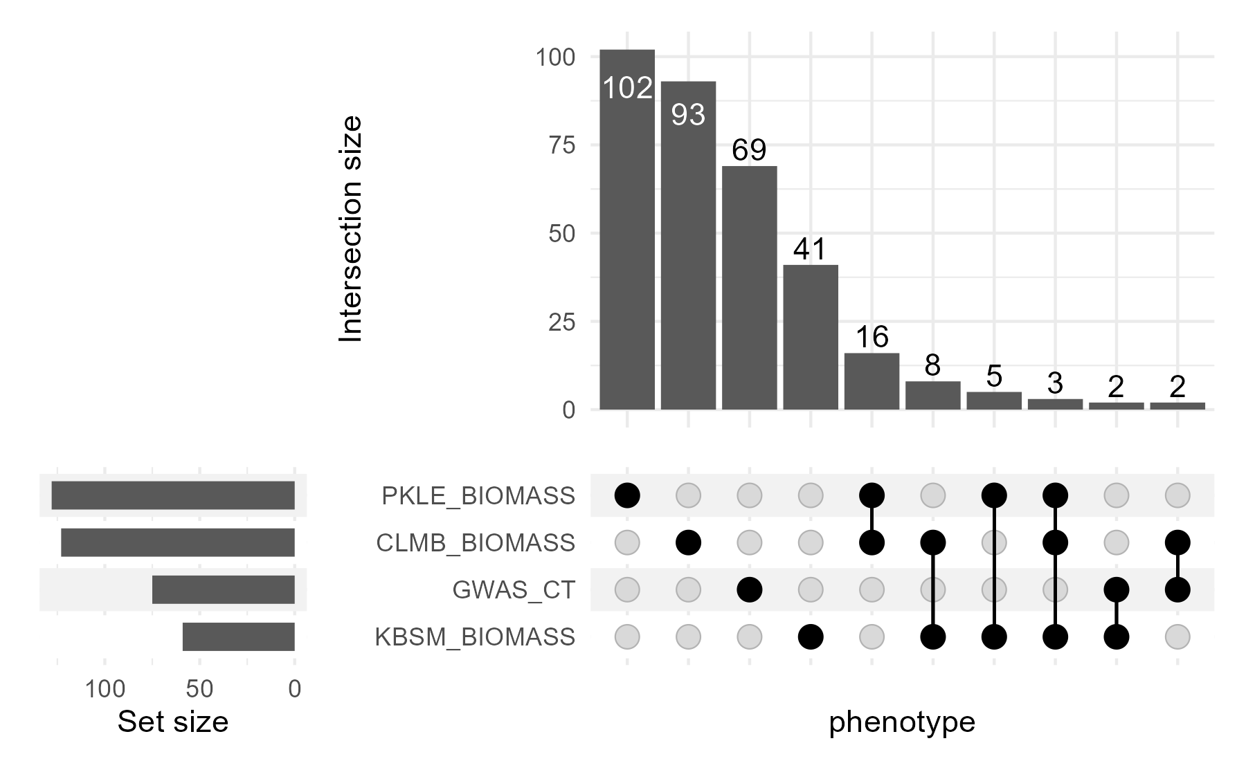

upset_ex In this Upset plot, we can see that there are many more SNPs significant in one or more biomass phenotype than there are significant for the phenotype ‘GWAS_CT’ and any biomass phenotype. Though, overall, most SNPs are significant in only one of the four conditions.

Sometimes this could be because different SNPs in the same gene or genomic region are coming up as highly associated with the different phenotypes. To test this, we can summarize our upset_df slightly based on position, and make a new Upset plot.

Median LD in switchgrass is between 20 and 25kb. Normally this is the largest genomic region I would make. However, for this toy example, we’ll make larger genomic regions of 1Mb.

library(dplyr)
#> 
#> Attaching package: 'dplyr'
#> The following objects are masked from 'package:stats':
#> 
#>     filter, lag
#> The following objects are masked from 'package:base':
#> 
#>     intersect, setdiff, setequal, union

upset_df_1Mb <- upset_df %>%
  mutate(POS_binned = floor(POS/1000000)*1000000) %>%
  select(-POS) %>%
  select(CHR, POS_binned, everything()) %>%
  group_by(CHR, POS_binned) %>%
  summarise(across(everything(), ~ max(.x)))
#> `summarise()` has grouped output by 'CHR'. You can override using the `.groups` argument.

upset_1Mb <- upset(upset_df_1Mb, intersect = colnames(upset_df_1Mb)[-(1:2)], 
                    name = 'phenotype', min_size = 2) + 
  labs(title = "Significant at -log10p > 2 in 1Mb intervals")
upset_1Mb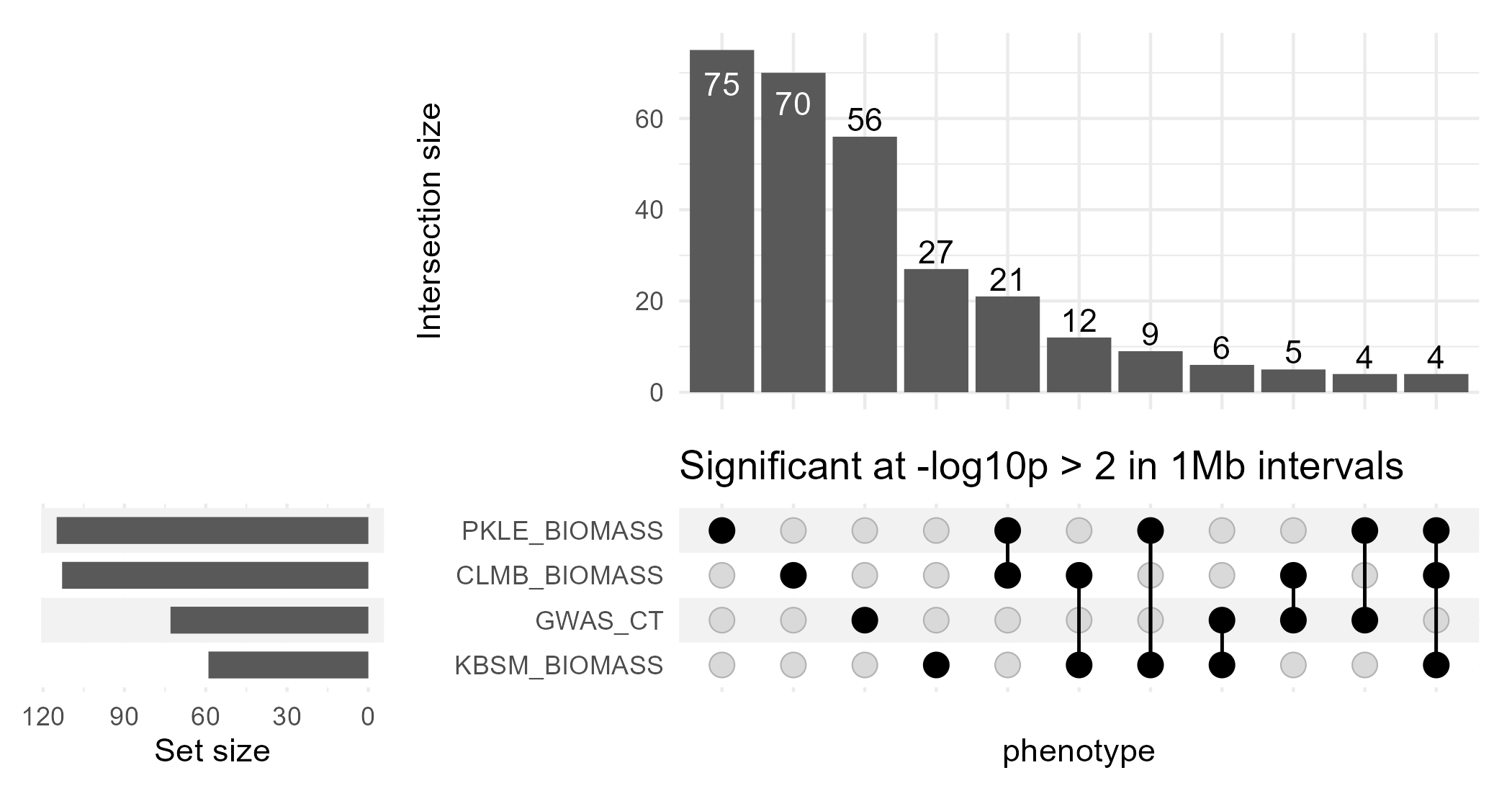

upset_ex

This binning by genomic interval does result in more genomic regions with significant effects on multiple phenotypes. It doesn’t change the ordering of the kinds of intersections very much, with the exception that the three-way intersection between the three biomass phenotypes is now the least common intersection (with 4 1Mb regions containing significant associations for all three phenotypes).

What if we want to learn more about these 4 1Mb regions? We can go back to our upset dataframes to extract these regions.

sel_reg_biomass <- upset_df_1Mb %>%
  filter(across(CLMB_BIOMASS:PKLE_BIOMASS, ~ .x == 1)) %>%
  mutate(Sel_region = paste(CHR, POS_binned, sep = "_"))

sel_snp_biomass <- upset_df %>%
  mutate(POS_binned = floor(POS/1000000)*1000000,
         Sel_region = paste(CHR, POS_binned, sep = "_")) %>%
  filter(Sel_region %in% sel_reg_biomass$Sel_region)

kable(sel_snp_biomass)

CHR	POS	CLMB_BIOMASS	KBSM_BIOMASS	PKLE_BIOMASS	POS_binned	Sel_region
Chr03K	2197885	1	1	1	2.0e+06	Chr03K_2e+06
Chr05K	12177803	1	1	1	1.2e+07	Chr05K_1.2e+07
Chr09K	45587560	1	1	1	4.5e+07	Chr09K_4.5e+07
Chr09N	11325811	0	0	1	1.1e+07	Chr09N_1.1e+07
Chr09N	11967533	1	1	0	1.1e+07	Chr09N_1.1e+07

If we were interested enough in these regions, we could also use this table to find annotations using pvdiv_table_topsnps().

sel_snp_annos <- sel_snp_biomass %>%
  mutate(start = POS - 10000,
         end = POS + 10000)  # get the 20kb surrounding each position, POS, in thr_dfB

library(AnnotationDbi)
library(VariantAnnotation)
txdb <- loadDb(file = "../../pvdiv-genome/Pvirgatum_516_v5.1.gene.txdb.sqlite")

sel_snp_annos <- pvdiv_table_topsnps(df = sel_snp_annos, type = "table", txdb = txdb)

kable(sel_snp_annos)

CHR	region_start	region_end	width	region_strand	Annotation	QUERYID	TXID	Gene ID	POS	CLMB_BIOMASS	KBSM_BIOMASS	PKLE_BIOMASS	POS_binned	Sel_region	gene_start	gene_end	gene_width	gene_strand	pacId	transcriptName	peptideName	Pfam	Panther Categories	KOG	ec	KO	GO	Arabidopsis thaliana homolog	A. thaliana gene name	A. thaliana gene annotation	Rice homolog	Rice gene name	Rice gene annotation	d2_start	d2_end	distance from gene
Chr03K	2187885	2207885	20001	*	intergenic	1	NA	NA	2197885	1	1	1	2.0e+06	Chr03K_2e+06	NA	NA	NA	NA	NA	NA	NA	NA	NA	NA	NA	NA	NA	NA	NA	NA	NA	NA	NA	NA	NA	NA
Chr05K	12167803	12187803	20001	+	spliceSite	2	60175	Pavir.5KG164407	12177803	1	1	1	1.2e+07	Chr05K_1.2e+07	12176848	12177263	416	+	41543573	Pavir.5KG164407.1	Pavir.5KG164407.1.p	NA	NA	NA	NA	NA	NA	NA	NA	NA	NA	NA	NA	955	540	540
Chr05K	12167803	12187803	20001	+	spliceSite	2	60176	Pavir.5KG164807	12177803	1	1	1	1.2e+07	Chr05K_1.2e+07	12185636	12186204	569	+	41549658	Pavir.5KG164807.1	Pavir.5KG164807.1.p	NA	NA	NA	NA	NA	NA	NA	NA	NA	NA	NA	NA	-7833	-8401	7833
Chr09K	45577560	45597560	20001	-	intron	3	103241	Pavir.8KG390800	45587560	1	1	1	4.5e+07	Chr09K_4.5e+07	NA	NA	NA	NA	41644684	Pavir.8KG390800.1	Pavir.8KG390800.1.p	PF03810	PTHR10997,PTHR10997:SF29	NA	NA	NA	GO:0008536,GO:0006886	AT3G17340.1	NA	ARM repeat superfamily protein	LOC_Os11g47320.1	NA	protein transporter, putative, expressed	NA	NA	NA
Chr09K	45577560	45597560	20001	+	spliceSite	3	110376	Pavir.9KG334200	45587560	1	1	1	4.5e+07	Chr09K_4.5e+07	45586592	45589853	3262	+	41604637	Pavir.9KG334200.1	Pavir.9KG334200.1.p	PF00249	PTHR24078,PTHR24078:SF195	NA	NA	NA	NA	AT5G47390.1	NA	myb-like transcription factor family protein	LOC_Os10g41200.1	NA	MYB family transcription factor, putative, expressed	968	-2293	968
Chr09K	45577560	45597560	20001	+	spliceSite	3	116062	Pavir.9KG334400	45587560	1	1	1	4.5e+07	Chr09K_4.5e+07	45576944	45582938	5995	-	41606480	Pavir.9KG334400.4	Pavir.9KG334400.4.p	PF00582,PF04564,PF00069	PTHR27003,PTHR27003:SF29	KOG1187	2.7.11.1	NA	GO:0006950,GO:0016567,GO:0004842,GO:0006468,GO:0005524,GO:0004672	AT4G25160.1	NA	U-box domain-containing protein kinase family protein	LOC_Os10g41220.1	NA	protein kinase family protein, putative, expressed	10616	4622	4622
Chr09K	45577560	45597560	20001	+	spliceSite	3	116063	Pavir.9KG334400	45587560	1	1	1	4.5e+07	Chr09K_4.5e+07	45576944	45582938	5995	-	41606480	Pavir.9KG334400.4	Pavir.9KG334400.4.p	PF00582,PF04564,PF00069	PTHR27003,PTHR27003:SF29	KOG1187	2.7.11.1	NA	GO:0006950,GO:0016567,GO:0004842,GO:0006468,GO:0005524,GO:0004672	AT4G25160.1	NA	U-box domain-containing protein kinase family protein	LOC_Os10g41220.1	NA	protein kinase family protein, putative, expressed	10616	4622	4622
Chr09K	45577560	45597560	20001	+	spliceSite	3	116064	Pavir.9KG334100	45587560	1	1	1	4.5e+07	Chr09K_4.5e+07	45590557	45594099	3543	-	41607551	Pavir.9KG334100.1	Pavir.9KG334100.1.p	PF07690	PTHR23500,PTHR23500:SF179	KOG0254	NA	NA	GO:0055085,GO:0016021	AT5G61520.1	NA	Major facilitator superfamily protein	LOC_Os10g41190.1	NA	transporter family protein, putative, expressed	-2997	-6539	2997
Chr09K	45577560	45597560	20001	+	spliceSite	3	116065	Pavir.9KG334100	45587560	1	1	1	4.5e+07	Chr09K_4.5e+07	45590557	45594099	3543	-	41607551	Pavir.9KG334100.1	Pavir.9KG334100.1.p	PF07690	PTHR23500,PTHR23500:SF179	KOG0254	NA	NA	GO:0055085,GO:0016021	AT5G61520.1	NA	Major facilitator superfamily protein	LOC_Os10g41190.1	NA	transporter family protein, putative, expressed	-2997	-6539	2997
Chr09K	45577560	45597560	20001	+	spliceSite	3	116066	Pavir.9KG334100	45587560	1	1	1	4.5e+07	Chr09K_4.5e+07	45590557	45594099	3543	-	41607551	Pavir.9KG334100.1	Pavir.9KG334100.1.p	PF07690	PTHR23500,PTHR23500:SF179	KOG0254	NA	NA	GO:0055085,GO:0016021	AT5G61520.1	NA	Major facilitator superfamily protein	LOC_Os10g41190.1	NA	transporter family protein, putative, expressed	-2997	-6539	2997
Chr09N	11315811	11335811	20001	-	intron	4	117033	Pavir.9KG583700	11325811	0	0	1	1.1e+07	Chr09N_1.1e+07	NA	NA	NA	NA	41598633	Pavir.9KG583700.1	Pavir.9KG583700.1.p	PF07716	PTHR22952,PTHR22952:SF198	NA	NA	NA	GO:0043565,GO:0006355,GO:0003700	AT3G62420.1	ATBZIP53,BZIP53	basic region/leucine zipper motif 53	LOC_Os03g19375.1	NA	expressed protein	NA	NA	NA
Chr09N	11315811	11335811	20001	+	spliceSite	4	124936	Pavir.9NG142800	11325811	0	0	1	1.1e+07	Chr09N_1.1e+07	11329238	11331352	2115	-	41552177	Pavir.9NG142800.1	Pavir.9NG142800.1.p	PF11250	PTHR33155,PTHR33155:SF1	NA	NA	NA	NA	AT5G22090.2	NA	Protein of unknown function (DUF3049)	LOC_Os03g49830.1	NA	expressed protein	-3427	-5541	3427
Chr09N	11315811	11335811	20001	+	spliceSite	4	124937	Pavir.9NG142800	11325811	0	0	1	1.1e+07	Chr09N_1.1e+07	11329238	11331352	2115	-	41552177	Pavir.9NG142800.1	Pavir.9NG142800.1.p	PF11250	PTHR33155,PTHR33155:SF1	NA	NA	NA	NA	AT5G22090.2	NA	Protein of unknown function (DUF3049)	LOC_Os03g49830.1	NA	expressed protein	-3427	-5541	3427
Chr09N	11957533	11977533	20001	+	intron	5	111994	Pavir.9KG622000	11967533	1	1	0	1.1e+07	Chr09N_1.1e+07	NA	NA	NA	NA	41599909	Pavir.9KG622000.1	Pavir.9KG622000.1.p	PF01588,PF09334	PTHR11946,PTHR11946:SF78	NA	6.1.1.10	K01874	GO:0000049,GO:0006418,GO:0005524,GO:0004812,GO:0000166	AT4G13780.1	NA	methionine–tRNA ligase, putative / methionyl-tRNA synthetase, putative / MetRS, putative	LOC_Os06g31210.1	NA	methionyl-tRNA synthetase, putative, expressed	NA	NA	NA
Chr09N	11957533	11977533	20001	+	spliceSite	5	119578	Pavir.9NG147300	11967533	1	1	0	1.1e+07	Chr09N_1.1e+07	11964735	11967667	2933	+	41554068	Pavir.9NG147300.1	Pavir.9NG147300.1.p	PF00227	PTHR11599,PTHR11599:SF6	KOG0177	3.4.25.1	K02734	GO:0051603,GO:0005839,GO:0004298	AT3G22630.1	PBD1,PRCGB	20S proteasome beta subunit D1	LOC_Os03g48930.1	NA	peptidase, T1 family, putative, expressed	2798	-134	134
Chr09N	11957533	11977533	20001	+	spliceSite	5	124997	Pavir.9NG147373	11967533	1	1	0	1.1e+07	Chr09N_1.1e+07	11967554	11968429	876	-	41561168	Pavir.9NG147373.1	Pavir.9NG147373.1.p	PF14368	PTHR33044,PTHR33044:SF14	NA	NA	NA	NA	AT2G48130.1	NA	Bifunctional inhibitor/lipid-transfer protein/seed storage 2S albumin superfamily protein	LOC_Os07g07860.1	NA	LTPL76 - Protease inhibitor/seed storage/LTP family protein precursor, expressed	-21	-896	21
Chr09N	11957533	11977533	20001	+	spliceSite	5	124998	Pavir.9NG147500	11967533	1	1	0	1.1e+07	Chr09N_1.1e+07	11968815	11969741	927	-	41554575	Pavir.9NG147500.1	Pavir.9NG147500.1.p	PF14368	PTHR33044,PTHR33044:SF14	NA	NA	NA	NA	AT3G22600.1	NA	Bifunctional inhibitor/lipid-transfer protein/seed storage 2S albumin superfamily protein	LOC_Os03g57970.1	NA	LTPL73 - Protease inhibitor/seed storage/LTP family protein precursor, expressed	-1282	-2208	1282
Chr09N	11957533	11977533	20001	+	spliceSite	5	124999	Pavir.9NG147573	11967533	1	1	0	1.1e+07	Chr09N_1.1e+07	11970419	11974568	4150	-	41553090	Pavir.9NG147573.1	Pavir.9NG147573.1.p	PF07466	PTHR33975,PTHR33975:SF2	NA	NA	NA	NA	AT1G54520.1	NA	NA	LOC_Os03g48920.1	NA	DUF1517 domain containing protein, putative, expressed	-2886	-7035	2886

Using file-backed matrices - FBM

Alice MacQueen

2022-01-13