Genome-Wide Association
Alice MacQueen
2020-01-06
gwas.RmdGet genotype file
# get the example bedfile from the package switchgrassGWAS
bedfile <- system.file("extdata", "example.bed", package = "switchgrassGWAS")
Set up SNP and phenotype data frames.
# Load packages bigsnpr and switchgrassGWAS
library(switchgrassGWAS)
#> Registered S3 method overwritten by 'GGally':
#>   method from
#>   +.gg   ggplot2
library(bigsnpr)
#> Loading required package: bigstatsr

# Read from bed/bim/fam to create the new files that bigsnpr uses.
# Let's put them in an temporary directory for this demo.
tmpfile <- tempfile()
snp_readBed(bedfile, backingfile = tmpfile)
#> [1] "/tmp/RtmpyiBzRL/file2fb621c0ae49.rds"

# Attach the "bigSNP" object to the R session.
snp_example <- snp_attach(paste0(tmpfile, ".rds"))
# What does the bigSNP object look like?
str(snp_example, max.level = 2, strict.width = "cut")
#> List of 3
#>  $ genotypes:Reference class 'FBM.code256' [package "bigstatsr"] with 16 fields
#>   ..and 26 methods, of which 12 are  possibly relevant:
#>   ..  add_columns, as.FBM, bm, bm.desc, check_dimensions,
#>   ..  check_write_permissions, copy#envRefClass, initialize, initialize#FBM,
#>   ..  save, show#envRefClass, show#FBM
#>  $ fam      :'data.frame':   630 obs. of  6 variables:
#>   ..$ family.ID  : chr [1:630] "Pvirgatum" "Pvirgatum" "Pvirgatum" "Pvirgatum"..
#>   ..$ sample.ID  : chr [1:630] "J181.A" "J250.C" "J251.C" "J352.A" ...
#>   ..$ paternal.ID: int [1:630] 0 0 0 0 0 0 0 0 0 0 ...
#>   ..$ maternal.ID: int [1:630] 0 0 0 0 0 0 0 0 0 0 ...
#>   ..$ sex        : int [1:630] 0 0 0 0 0 0 0 0 0 0 ...
#>   ..$ affection  : int [1:630] -9 -9 -9 -9 -9 -9 -9 -9 -9 -9 ...
#>  $ map      :'data.frame':   3600 obs. of  6 variables:
#>   ..$ chromosome  : chr [1:3600] "Chr01K" "Chr01K" "Chr01K" "Chr01K" ...
#>   ..$ marker.ID   : chr [1:3600] "Chr01K_105542" "Chr01K_798650" "Chr01K_1147"..
#>   ..$ genetic.dist: int [1:3600] 0 0 0 0 0 0 0 0 0 0 ...
#>   ..$ physical.pos: int [1:3600] 105542 798650 1147074 1719551 1915851 1965986..
#>   ..$ allele1     : chr [1:3600] "A" "C" "T" "T" ...
#>   ..$ allele2     : chr [1:3600] "G" "G" "C" "G" ...
#>  - attr(*, "class")= chr "bigSNP"

# Load the pvdiv phenotypes into the R session.
data(pvdiv_phenotypes)
# Make an example dataframe of one phenotype where the first column is PLANT_ID.
# This "phenotype", 'GWAS_CT', is the number of times a plant successfully
# clonally replicated to plant in the common gardens in 2018.
one_phenotype <- pvdiv_phenotypes %>%
  dplyr::select(PLANT_ID, GWAS_CT)
Run genome-wide association (GWAS)
# Save the output to a temporary directory for this demo.
tempdir <- tempdir()

pvdiv_standard_gwas(snp = snp_example, df = one_phenotype,
                    type = "linear", outputdir = tempdir,
                    savegwas = FALSE, saveplots = TRUE,
                    saveannos = FALSE, ncores = 1)
#> 'lambdagc' is TRUE, so lambda_GC will be used to find the best population structure correction using the covariance matrix.
#> 'savegwas' is FALSE, so the gwas results will not be saved to disk.
#> Covariance matrix (covar) was not supplied - this will be generated using pvdiv_autoSVD().
#> 'saveoutput' is FALSE, so the svd will not be saved to the working directory.
#> Now starting GWAS pipeline for GWAS_CT.
#> Now determining lambda_GC for GWAS models with 16 sets of PCs. This will take some time.
#> saveoutput is FALSE, so lambda_GC values won't be saved to a csv.
#> Finished Lambda_GC calculation for GWAS_CT using 0 PCs.
#> Finished Lambda_GC calculation for GWAS_CT using 1 PCs.
#> Finished Lambda_GC calculation for GWAS_CT using 2 PCs.
#> Finished Lambda_GC calculation for GWAS_CT using 3 PCs.
#> Finished Lambda_GC calculation for GWAS_CT using 4 PCs.
#> Finished Lambda_GC calculation for GWAS_CT using 5 PCs.
#> Finished Lambda_GC calculation for GWAS_CT using 6 PCs.
#> Finished Lambda_GC calculation for GWAS_CT using 7 PCs.
#> Finished Lambda_GC calculation for GWAS_CT using 8 PCs.
#> Finished Lambda_GC calculation for GWAS_CT using 9 PCs.
#> Finished Lambda_GC calculation for GWAS_CT using 10 PCs.
#> Finished Lambda_GC calculation for GWAS_CT using 11 PCs.
#> Finished Lambda_GC calculation for GWAS_CT using 12 PCs.
#> Finished Lambda_GC calculation for GWAS_CT using 13 PCs.
#> Finished Lambda_GC calculation for GWAS_CT using 14 PCs.
#> Finished Lambda_GC calculation for GWAS_CT using 15 PCs.
#> Finished phenotype 1: GWAS_CT
#> Now running GWAS with the best population structure correction.
#> [1] "saveoutput is FALSE so GWAS object will not be saved to disk."
#> Now generating and saving Manhattan and QQ plots.
This command will save a Manhattan and QQ-plot for the ~1800 SNPs from the example file to a temporary directory, which will have a randomly generated name like: /tmp/RtmpyiBzRL.
The example Manhattan plot should look like this:
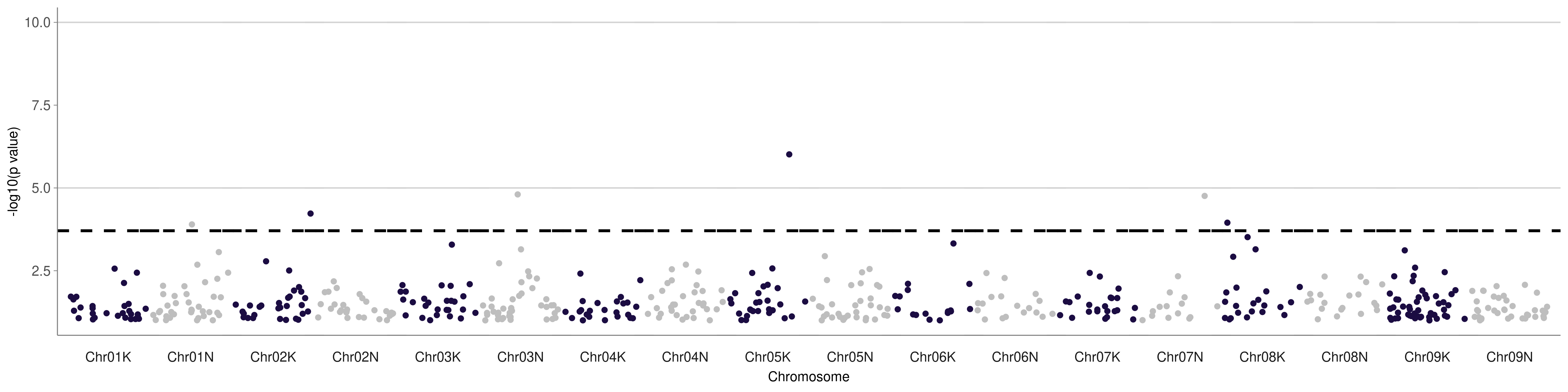
Manhattan
And the example QQ plot should look like this.
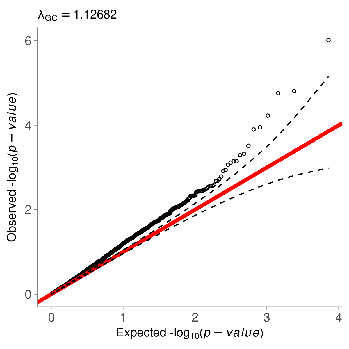
QQ-plot
pvdiv_standard_gwas is a wrapper function for the standard GWAS done in the Juenger lab. You must specify three things to use this function: 1) a snp file in bigSNP format, 2) a phenotype file where the first column is PLANT_ID (as in switchgrassGWAS::pvdiv_metadata), and 3) whether the GWAS should be a linear or logistic regression.
Additional features:
* Specify `savegwas = TRUE` if you want the GWAS outputs to be saved to the output directory as .rds files.
* Specify `saveplots = TRUE` if you want Manhattan and QQ-plots to be generated and saved to the output directory. (NB: This is the default.)
* Specify `saveannos = TRUE` and specify a txdb object loaded into your environment with AnnotationDbi::loadDb, if you want annotation tables for top SNPs to be generated and saved to the output directory.
* Specify an integer value for `minphe` if you want to specify a minimum number of phenotyped individuals to conduct a GWAS on.
Troubleshooting:
If you get the error “Error in snp_autoSVD(G = G, infos.chr = CHRN$CHRN, infos.pos = POS, ncores = ncores, : object ‘LD.wiki34’ not found”
Likely you have not called library(bigsnpr) in your current R session. You may need to run install.packages("bigsnpr") and then library(bigsnpr), then try running the pvdiv_standard_gwas() command again.
If you cannot find the temporary directory you created (tempdir): Try setting the output directory (outputdir) to your current working directory using outputdir = “.” within pvdiv_standard_gwas(), or tempdir <- “.” & keeping the pvdiv_standard_gwas() function as-is, then try running the pvdiv_standard_gwas() command again.