Multivariate Adaptive Shrinkage

Alice MacQueen

2020-01-06

Analysis of multiple phenotypes or planting locations

Many researchers are measuring phenotypes on the Panicum virgatum diversity panel to understand the genes and genetic regions affecting these phenotypes. When similar phenotypes are collected at many locations, researchers may be interested in the extent to which effects of SNPs are similar or different across these different locations. The R package mashr can be used to conduct this kind of analysis, and downstream plotting functions in switchgrassGWAS can be used to further visualize and interpret the results of this analysis.

After you run your GWAS using bigsnpr, there are three steps to running a mash analysis. First, you must convert the bigsnpr results to mashr input format. Second, you run the mash analysis. Third, you can visualize the mash results using mashr functions or using functions from switchgrassGWAS.

1. Run pvdiv_bigsnp2mashr function

The first three commands are setup for running the pvdiv_bigsnp2mashr function.

You want a character vector containing the names of the rds files containing your GWAS results - you can find that with list.files() or with pvdiv_results_in_folder(). The path should be the location of the gwas files, and can be a relative or absolute path. The pattern to match can be anything, but defaults to "*.rds". Here I have used regular expressions to find four files to demonstrate mashr on.

Second, you what a character vector the same length as the one containing your GWAS rds files. This contains strings of whatever you want your phenotypic column names to ultimately be. If you’ve put the phenotype name into the GWAS rds file name (which I’d certainly recommend!), you can find this with a str_sub() command.

Third, you want to calculate the number of SNPs with low p-values to select from each GWAS. Ideally mash will have from 1-2M cells for reasonable run times. You can divide 2 million by the square of the number of phenotypes you have to get a reasonable starting point for this value. Depending on your computing power and the amount of overlap of low p-value SNPs between your GWAS, you may need to tweak this number further.

Finally, you run the pvdiv_bigsnp2mashr() function using these quantities. Choose the model type that you ran on your GWAS. Current options are “logistic” or “linear”. Mixing these types is not supported (and statistically is probably a bad idea, also.) Also choose whether you want to save the output to a file in your path - recommended, though the default is FALSE, so the user needs to ‘opt in’ to this.

data(pvdiv_phenotypes)
gwas <- pvdiv_gwas(df = pvdiv_phenotypes, type = "linear",
                   snp = snp, covar = svd0, ncores = NCORES)


load("markers.rda")
load("markers2.rda")
snp <- snp_attach("Pvirgatum_4x_784g_imp_phased_maf0.02_QC.rds")
G <- snp$genotypes
gwas_rds <- pvdiv_results_in_folder(path = ".", pattern = "GWAS_object_")

phenotype_names <- str_sub(gwas_rds, start = 13, end = -5)

numSNPs <- ceiling(1500000/length(phenotype_names)^2)

mash_input <- bigsnp2mashr(path = ".", gwas_rds = gwas_rds, 
                           phenotypes = phenotype_names, numSNPs = numSNPs, 
                           markers = markers, markers2 = markers2, G = G, 
                           model = "linear", saveoutput = TRUE)

2. Run a standard mash analysis

Here, the input is the list object you obtained from bigsnp2mashr() in the previous step. Again, you can choose to save the output to a file in your path. You can optionally specify numSNPs, or if you are running this in a session where you don’t have the output from bigsnp2mashr() in your environment, you can specify numSNPs equivalent to your bigsnp2mashr() run and this function will find the rds files it saved (on that path, with that number of SNPs) for you.

mash_output <- mash_standard_run(path = ".", list_input = mash_input, 
                                  numSNPs = numSNPs, saveoutput = TRUE)

# Or, if you are doing this in a new session and don't have mash_input 
#     in your workspace, you just need to enter the number of SNPs and this 
#     function will find a previously saved rds file with that numSNPs for you:
# mash_output <- mash_standard_run(path = ".", numSNPs = numSNPs,
#                                  saveoutput = TRUE)

3. Visualize mash output

You have a lot of options here, and some great ones (most importantly, mash_plot_meta) are already included in the mashr package.

However, this package adds a few additional options for viewing mash outputs.

3a. Number of Significant SNPs per Number of Conditions

This plot can help answer questions like, “at how many planting sites do SNPs affect this phenotype?”

nbycond <- mash_plot_sig_by_condition(m = mash_output)
nbycond$ggobject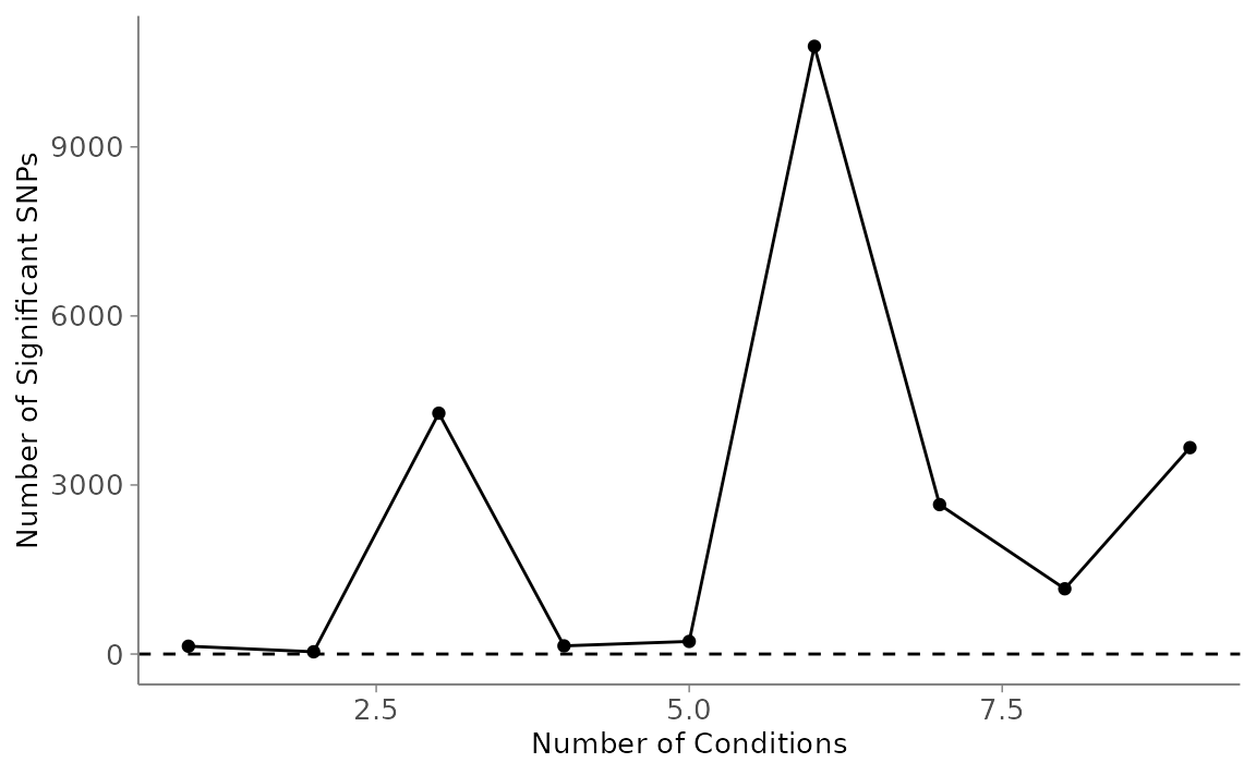

3b. Manhattan-esque plot (“Mashhattan”)

This plot can help answer questions like, “What is the genomic distribution of SNPs with significant effects, and at how many planting sites do these SNPs affect the phenotype?”

mashhattan <- mash_plot_manhattan_by_condition(m = mash_output)
mashhattan$ggmanobject
#> Warning: It is deprecated to specify `guide = FALSE` to remove a guide. Please
#> use `guide = "none"` instead.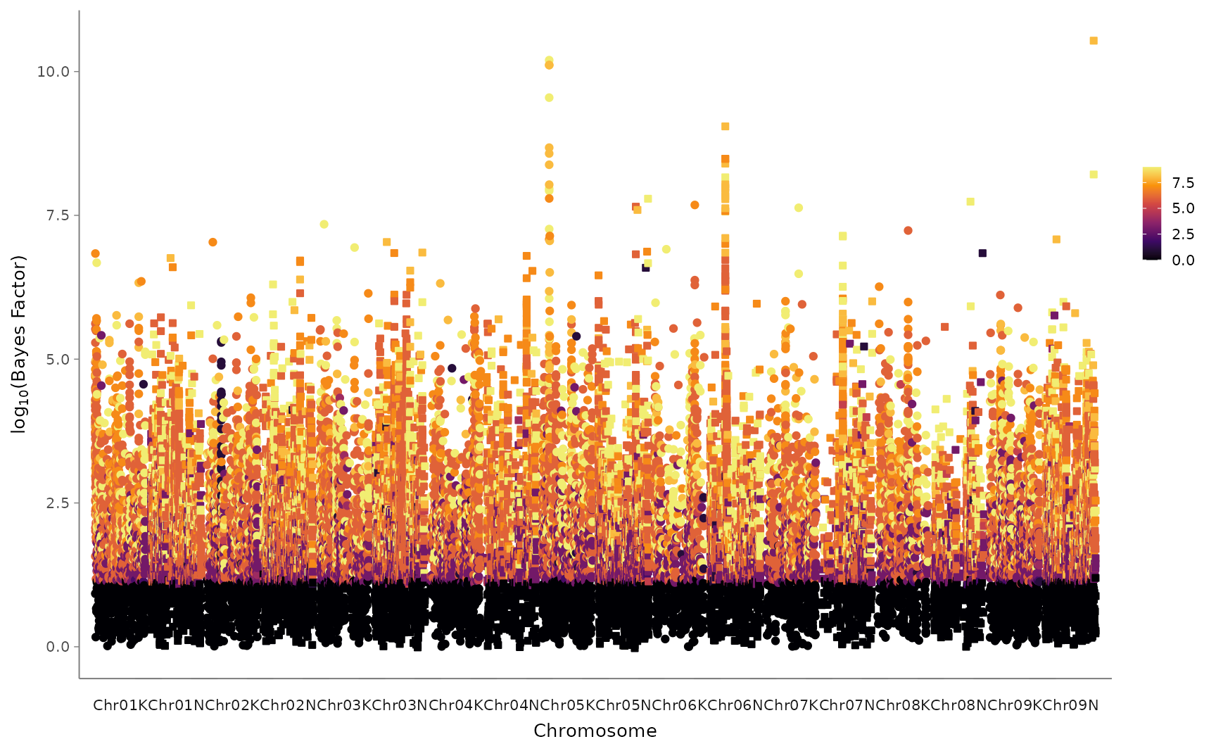

3c. Pairwise sharing of similar effects

This plot can help answer questions like, “How many SNPs have similar effects at pairs of planting sites?”. As most analyses of GxE typically only consider interactions between pairs of sites, this plot is a useful extension of two-site models.

If you saved the output of a mash_standard_run(), then you have saved two get_pairwise_sharing() outputs as rds objects already. All you need to do then is tell this function 1) the path to the RDS, for effectRDS; or 2) the correlation matrix you’re using if it’s an object in your environment, for corrmatrix.

pairwise_plot <- mash_plot_pairwise_sharing(effectRDS = pairwisefilepath,
                                            reorder = TRUE) 
#> Scale for 'colour' is already present. Adding another scale for 'colour',
#> which will replace the existing scale.
pairwise_plot$gg_corr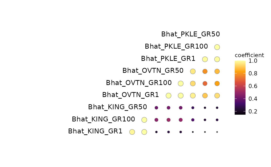

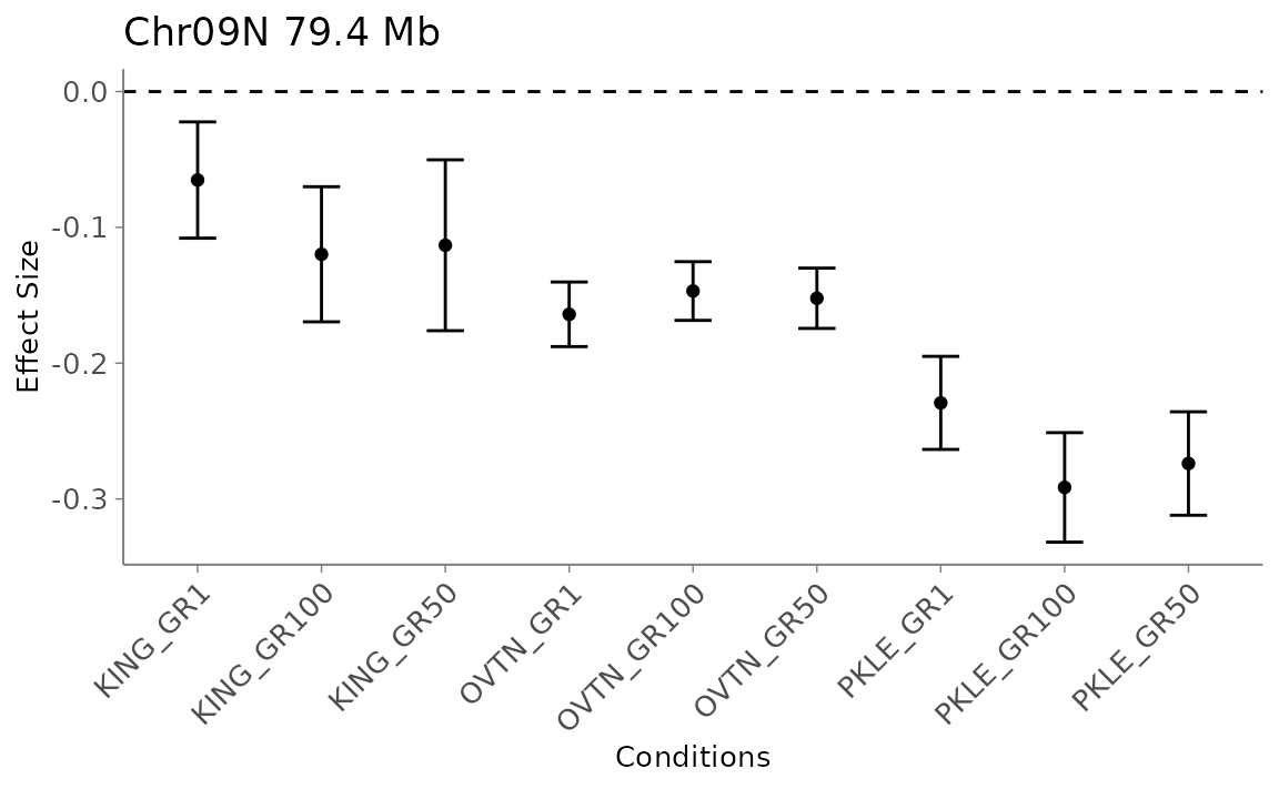
3d. Look at mash effect plots

This plot can help answer questions like, “What are the effects of a single SNP on the phenotype across planting sites?”

This will return ggplot objects for the effect plots for the nth significant SNP, ranked by the most significant local false sign rate. You can find the names of the top ten effects, for example, using get_significant_results(m = mashoutput)[1:10].

Alternatively, if you have the row number of the SNP you want to plot (which you can find with get_marker_df()), you can put that in as i.

effects <- mash_plot_effects(m = mash_output, n = 1)
effects$ggobject